How to design a polynomial that does what you want
2025-10-16
The other day, for a work thing, I needed a function that would smoothly interpolate between two values over a unit interval. For a smooth transition between two values, a sigmoid is often a good choice. However, the sigmoid never becomes perfectly flat on either side. I wanted a function that would have a continuous first derivative: it should smoothly approach the point \( (0, 0) \), and have a zero first derivative there. Similarly on the other side, it should approach \( (1, 1) \) and have a zero derivative there as well. We're looking for a function $f$ that satisfies \begin{align*} f(0) &= 0 \qquad &&f(1) = 1 \\ f'(0) &= 0 \qquad &&f'(1) = 0 \end{align*}
After designing a polynomial with these properties, I immediately realized that I could have just gone with a shifted and scaled sine function. But the process I used to design it deserves a writeup, since it illuminates some fundamentals of polynomial approximation.
In short, we construct a linear system whose solution is the vector of coefficients of a polynomial with the desired property. There are four constraints: a function value and a derivative at each of the two endpoints. That tells us we should expect a unique combination of four coefficients to solve the problem, i.e. a cubic polynomial:
\begin{align*} f(x) = ax^3 + bx^2 + cx + d \end{align*}
Our first constraint, \( f(0) = 0 \), can be expressed as a vector-vector product like so: \begin{align*} \begin{pmatrix} 0^3 & 0^2 & 0^1 & 1 \end{pmatrix} \cdot \begin{pmatrix} a \\ b \\ c \\ d \end{pmatrix} = 0 \end{align*}
The derivative constraints have a slightly different form, which we can read off from the expression for \( f'(x) \): \begin{align*} f'(x) = 3ax^2 + 2bx + c. \end{align*} With this in mind you should be able to construct the equation for \( f'(1) = 1 \): \begin{align*} \begin{pmatrix} 3 (1^2) & 2 (1^1) & 1 & 0 \end{pmatrix} \cdot \begin{pmatrix} a \\ b \\ c \\ d \end{pmatrix} = 0. \end{align*}
If we stack all four of the constraint equations into a matrix-vector product, we get \begin{align*} \begin{pmatrix} 0^3 & 0^2 & 0^1 & 1 \\ 1^3 & 1^2 & 1^1 & 1 \\ 3 (0^2) & 2 (0) & 0 & 0 \\ 3 (1^2) & 2 (1) & 1 & 0 \end{pmatrix} \cdot \begin{pmatrix} a \\ b \\ c \\ d \end{pmatrix} = \begin{pmatrix} 0 \\ 1 \\ 0 \\ 0 \end{pmatrix}. \end{align*}
Here's a Python program to construct and solve this linear system:
L = 0.0
R = 1.0
vand = np.array([
    [L**3, L**2, L, 1.0],
    [R**3, R**2, R, 1.0],
    [3*L**2, 2*L, 1.0, 0.0],
    [3*R**2, 2*R, 1.0, 0.0],
])
vals = np.array([0.0, 1.0, 0.0, 0.0])

coefs = np.linalg.solve(vand, vals)
a, b, c, d = coefs
I've named the matrix vand because it's a form of a Vandermonde matrix---really, two stacked Vandermonde matrices, one for \( f(x) \) and one for \( f'(x) \), at the points 0 and 1.
Solving this linear system gives the cubic polynomial we want: \begin{align*} f(x) = -2x^3 + 3x^2. \end{align*}
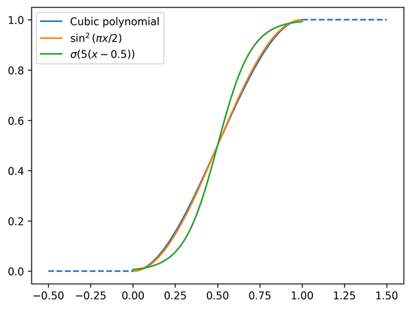
Let's compare the result to either of the transcendental options that come to mind. The sigmoid function does a quite bad job at this task. If we want to make the endpoints smoother, we'll need to make the central transition even steeper. Our cubic polynomial matches the sinusoid interpolant quite closely. If you just want a smooth function with these properties, the two-term polynomial might be more efficient to evaluate than the sinusoid.
This is quite a simple application of Vandermonde matrices, but the same ideas underly much more sophisticated numerical tools, from chebfun to high-order finite element analysis. The core analytical method we used here is probably the single most important idea in applied mathematics: figure out how to express your problem as a system of linear equations. Once you've done that, you can solve anything.